Numerical study of experimentally inspired stratified turbulence forced by waves
Internal gravity wave turbulence in the lab?
Oceanic and atmospheric measurements interpreted as IGW turbulence
Reproducible in the lab?
Stable density stratification $\Rightarrow$ Waves (IGW) and "vortices" ($\omega_z$)
Stratified turbulence (forced by vortices)
Horizontal Froude number $F_h$ and buoyancy Reynolds number $\R = Re {F_h}^2$
LAST regime $F_h<0.02$, $\R>20$: downscale energy cascade and anisotropic spectra
$\R = Re {F_h}^2 > 20 \Rightarrow Re \gg 1$
- experiments: very large apparatus
- simulations: high resolution
Internal gravity wave turbulence in the Coriolis facility!
Coriolis platform in Grenoble
- 13m-diameter, 1m-deep, 130 tons water
- stratification with salt
rotation up to 6 rpm

Internal gravity wave turbulence in the Coriolis facility!


Linearly stratified ($\sim$ 1 ton of salt)
Savaro et al. PRFluids 2020

Numerical setup: experimentally inspired stratified turbulence forced by waves
Pseudo spectral solver
ns3d.stratof the open-source CFD framework Fluidsim3D periodic!

Basically same parameters than for the experiments in the Coriolis platform: size, viscosity, Brunt-Väisälä frequency $N=0.6$ rad/s, forcing frequency $\omega_f = 0.73 N$ and forcing amplitude.
$\Rightarrow$ high resolution (up to $2304\times2304\times384$) and very long time (typically 15 h)
Numerical setup: experimentally inspired stratified turbulence forced by waves
 $2\pi / N \simeq 10$ s, $2\pi / \omega_f \simeq 15$ s
Long simulations at different resolution ($240\times240\times40$, $480\times480\times80$, $1152\times1152\times192$ and $2304\times2304\times384$)
Hyper viscosity is decreased when resolution is increased
$2304\times2304\times384$ quasi DNS
Strong vortical flow!
Stationarity?
Response to the forcing: $U_h$ and $\varepsilon_K$
$\Rightarrow F_h \simeq 6.5 \times 10^{{-4}}$ (strongly stratified) and $\R = Re {F_h}^2 \simeq 0.5$ (viscosity affected regime)
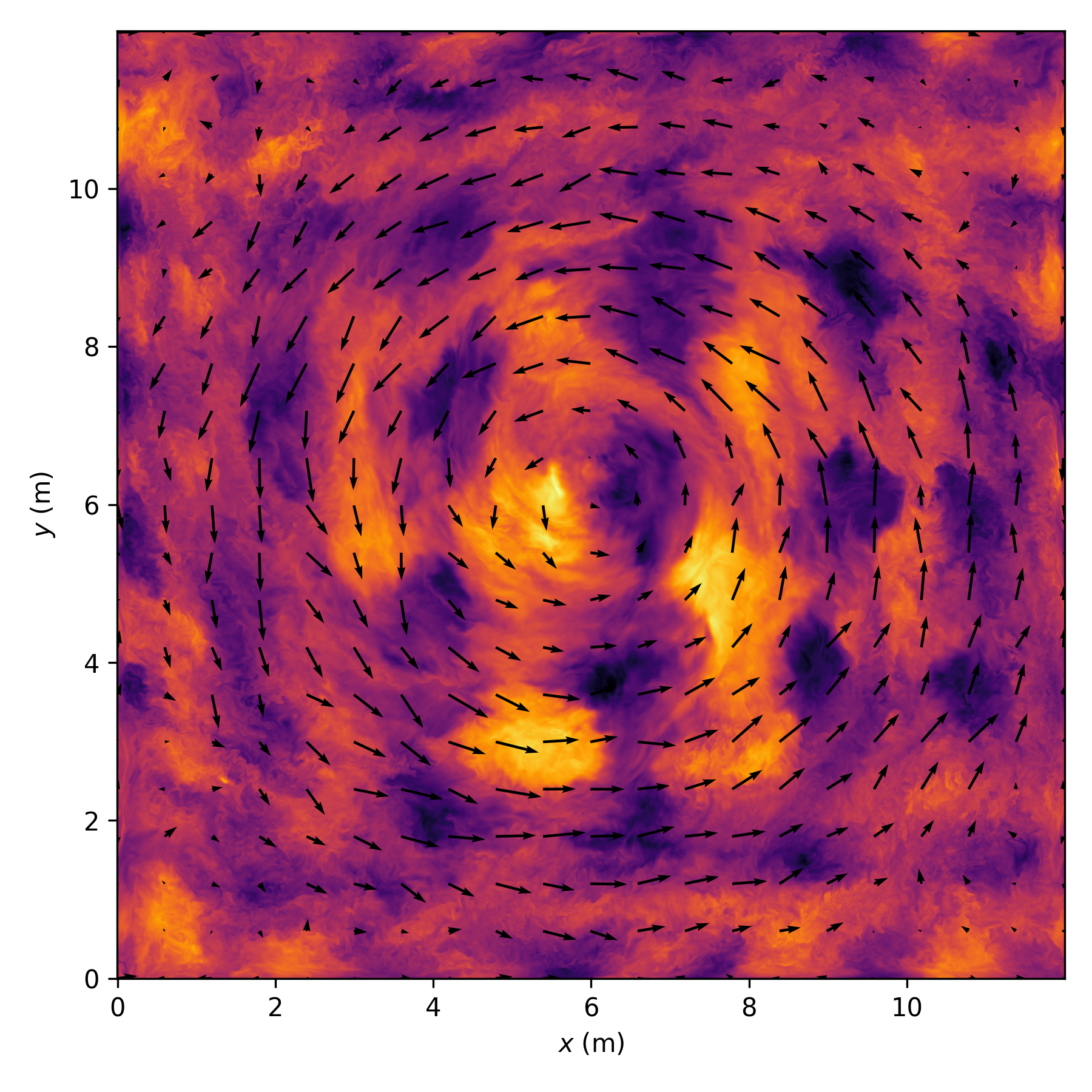
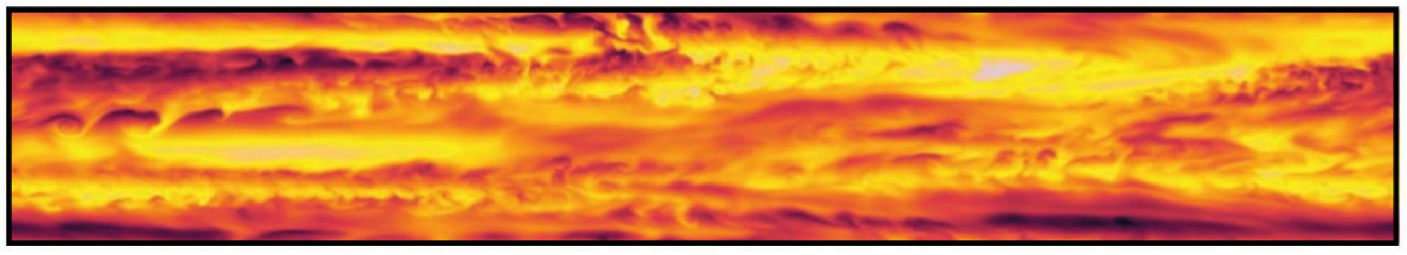
Snapshots for $\omega_f = 0.73N$ and $a = 5$ cm


large scale waves
small scale "turbulence"
thin vertical layers
2 counter-rotating vortices


Temporal spectra for $\omega_f = 0.73 N$ and $a = 5$ cm

Triads involving the forced frequency and modes of the numerical domain
Vortical flow dominates at very small frequency
Continuum between the peaks
Spatial spectra for $\omega_f = 0.73 N$ and $a = 5$ cm

Very strongly anisotropic spectra ("strongly stratified", $F_h \ll 10^{-2}$)
Viscosity affected flow ($\R \simeq 0.5$) but not far from the transition $\R > 1$
Spatio-temporal spectra for $\omega_f = 0.73 N$ and $a = 5$ cm

Triad: $\omega_1 + \omega_2 = \omega_f$ and $\vec{k}_1 + \vec{k}_2 = \vec{k}_f$
Spatio-temporal spectra for $\omega_f = 0.73 N$ and $a = 5$ cm


Weakly non linear waves only for first vertical modes
Stronger forcing for $\omega_f = 0.73 N$: $a=10$ cm


Conclusions
Pseudo spectral 3D periodic simulations with penalization can reproduce some aspects of the dynamics observed in experiments
The buoyancy Reynolds number $\R$ is crucial (transition at $\R \gtrsim 1$)
Accumulation of energy at large scales (2 counter-rotating vortices and waves)
Tank and forcing geometry $\Rightarrow$ normal modes ($\neq$ solutions for exp. and simulations...)
"Wave turbulence" between the modes
Not far from $\omega^{-2}$ between $\omega_f$ and $N$
Note: Fluidsim (https://fluidsim.readthedocs.io) is now a great tool!
conda create -n env-fluidsim ipython fluidsim "fluidfft[build=mpi*]" "h5py[build=mpi*]"