Studying mixing efficiency and stratified turbulence with experiments and open-science
$\newcommand{\kk}{\boldsymbol{k}} \newcommand{\eek}{\boldsymbol{e}_\boldsymbol{k}} \newcommand{\eeh}{\boldsymbol{e}_\boldsymbol{h}} \newcommand{\eez}{\boldsymbol{e}_\boldsymbol{z}} \newcommand{\cc}{\boldsymbol{c}} \newcommand{\uu}{\boldsymbol{u}} \newcommand{\vv}{\boldsymbol{v}} \newcommand{\bnabla}{\boldsymbol{\nabla}} \newcommand{\Dt}{\mbox{D}_t} \newcommand{\p}{\partial} \newcommand{\R}{\mathcal{R}} \newcommand{\eps}{\varepsilon} \newcommand{\mean}[1]{\langle #1 \rangle} \newcommand{\epsK}{\varepsilon_{\!\scriptscriptstyle K}} \newcommand{\epsA}{\varepsilon_{\!\scriptscriptstyle A}} \newcommand{\epsP}{\varepsilon_{\!\scriptscriptstyle P}} \newcommand{\epsm}{\varepsilon_{\!\scriptscriptstyle m}} \newcommand{\CKA}{C_{K\rightarrow A}} \newcommand{\D}{\mbox{D}}$


- LEGI group: Pierre Augier, A. Campagne, J. Sommeria, S. Viboud, C. Bonamy, N. Mordant...
- KTH group (Stockholm, Sweden): E. Lindborg, A. Vishnu, A. Segalini
- Diane Micard (LMFA)
Mixing efficiency and mixing coefficient
$$Ri_f \equiv \frac{\eps_P}{\eps_K + \eps_P} \quad \mbox{ and } \quad \Gamma \equiv \frac{\eps_P}{\eps_K},$$where $\eps_P$ and $\eps_K$ are the potential and kinetic energy dissipation.
Simple case: mixing a stably stratified fluid by stirring

stirring: injection of kinetic energy ($P_K$)
conversion from kinetic energy to potential energy (buoyancy flux) $- \mean{b w} = C_{K\rightarrow A} = \eps_P$
dissipation of kinetic and potential energy $\eps_K + \eps_P = P_K$
energy spent for mixing = dissipation of potential energy
Navier-Stokes equations under Boussinesq approximation
$$\begin{align} \D_t \vv &= -\bnabla p_{tot} + b_{tot} \eez + \mathbf{F} + \nu \bnabla^2 \vv,\\ \D_t b_{tot} &= \kappa \bnabla^2 b_{tot}, \end{align}$$where
- $\bnabla \cdot \vv = 0$,
- $b_{tot} = -\frac{g}{\rho_0} (\rho_0 + \int_{z_0}^z d_z\bar\rho dz + \rho) = -g + N^2 (z -z_0) + b$,
- $N^2 = d_z\bar b_{tot}$ the Brunt-Väisälä frequency is constant (linearly stratified)
Energetic
- Kinetic energy $\mathcal{E}_K = \mean{\vv^2}/2$
- Potential energy $\mathcal{E}_P = \mean{\rho g z/ \rho_0} = -\mean{b_{tot} z}$
$$ \mathcal{E}_P = -\frac{(HN)^2}{12} - \mean{b z}. $$
Available Potential Energy (APE)
$$\mathcal{E}_P + \frac{(HN)^2}{12} = \mean{b z}$$
- Equations for the buoyancy fluctuations $b$
$$\begin{align} \D_t \vv &= -\bnabla p + b\eez + \mathbf{F} + \nu \bnabla^2 \vv \\ \D_t b &= - N^2 w + \kappa \bnabla^2 b \end{align}$$
- Density of APE $E_A$:
$$\begin{align} d_t E_K &= -\bnabla \cdot (p \vv) - \CKA - \epsK\\ d_t E_A &= \CKA - \epsA \end{align}$$
where
- $E_K = \vv^2/2$,
- $E_A = b^2/(2N^2)$,
- $\epsK = - \nu \vv \cdot \bnabla^2 \vv$,
- $\epsA = - \kappa b \cdot \bnabla^2 b$,
- $\CKA = - b w$
Why is the mixing coefficient $\Gamma$ important?
Ocean models are LES (scale filter $[]$).
- Approximation of a term similar to a Reynolds stress with a turbulent diffusivity
- Approximation of the turbulent diffusivity from a flux law for the buoyancy flux:
- Approximation of the energy conversion $\CKA$ by a proportionality relation
with $\Gamma = 0.2$ a constant!
But actually $\Gamma$ is not really a constant!
And this has consequences for the large-scale results of the ocean models!
We need better parametrization of the mixing
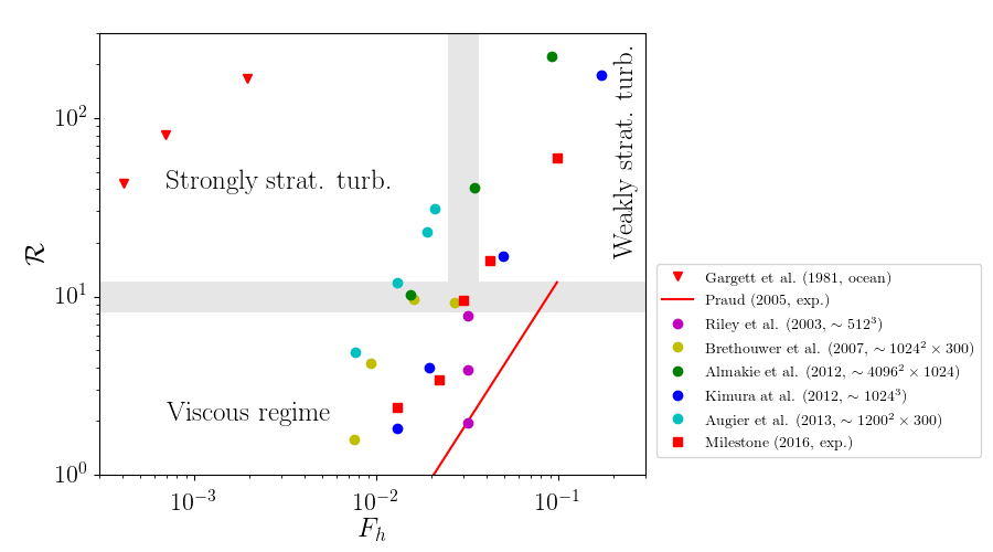
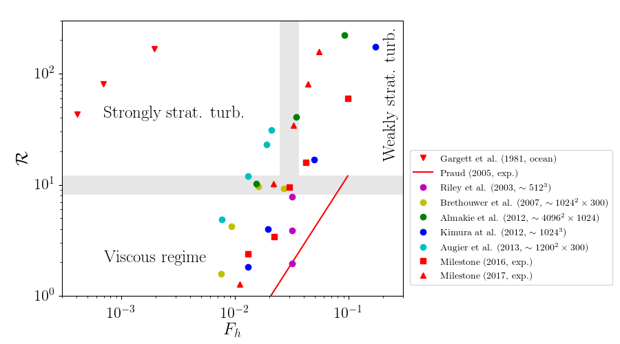
Stratified flows and their different régimes
Introduction of 2 important non-dimensional numbers
- horizontal Froude number $F_h$
- buoyancy Reynolds number $\R$
Strongly anisotropic flows


- low vertical velocity
- vertical length scale $L_v \ll$ horizontal length scale $L_h$
- $L_v \sim$ buoyancy length scale $L_b = U/N $, where $U$ is the characteristic horizontal velocity
Influence of the stratification, horizontal Froude number $F_h$
$$F_h = \frac{U}{NL_h} = \frac{L_b}{L_h} < 1$$
Theory of "strongly stratified turbulence"
Linborg (2006)

($E_K$ and $E_A$)
Different scales:
buoyancy length scale $L_b=U/N$
-
Ozmidov length scale $l_o= (\varepsilon_K/N^3)^{1/2}$
"the largest horizontal scale that can overturn" (Riley & Lindborg, 2008)
-
Kolmogorov length scale $\eta$ (dissipative structures)
Viscous condition $l_o \gg \eta$
buoyancy Reynolds number $$\displaystyle \R = \left( \frac{l_o}{\eta} \right)^{4/3} \sim Re {F_h}^2 \gg 1$$
Order of magnitude of $F_h$ and $Re$
In the oceans and the atmosphere, $L_h \gg 1$ so that $F_h \ll 1$ and $\R \gg 1$
DNS fine resolution ($\sim 10^3 \times 10^3 \times 10^2$ grid points): $\R \simeq 10$

In the laboratory experiments
In water with stratification with salt $\Rightarrow N \simeq 1$ rad/s and $\nu \simeq 10^{-6}$ m$^2$/s
$F_h = \frac{U}{L_hN} \ll 1 \Rightarrow$ slow motion
$\R = Re {F_h}^2 \gg 1 \Rightarrow$ need very large $Re$
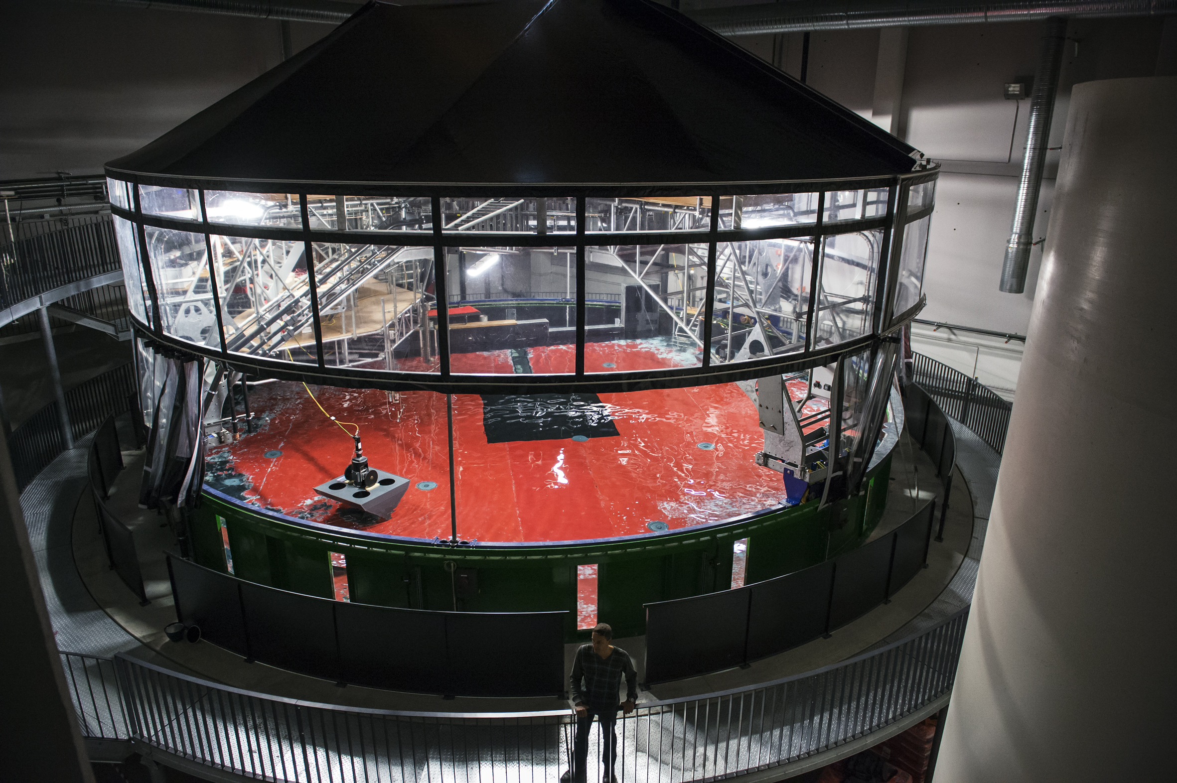
Large Reynolds + slow motion $\Rightarrow$ very large apparatus
Flow regimes in stratified fluids in the $[F_h,\ \R]$ parameter space
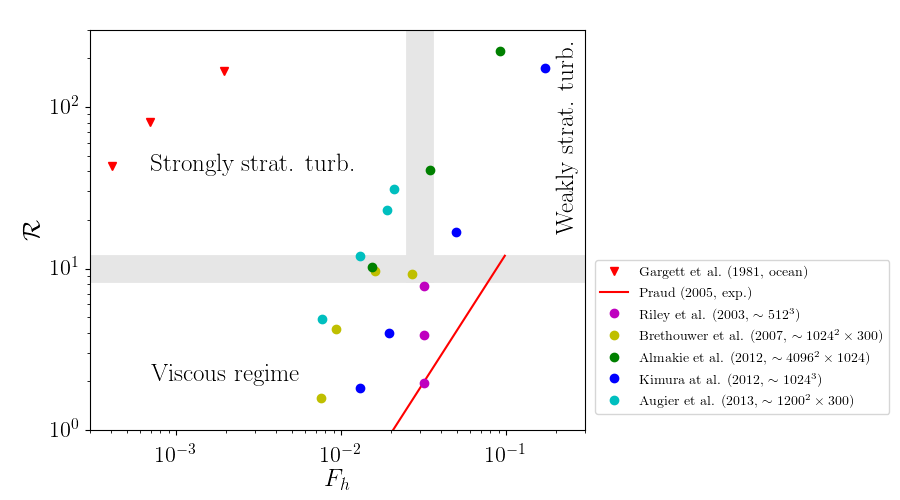
Scaling laws for the mixing coefficient in the different turbulent régimes
- Weakly stratified turbulence (passive scalar)
- Strongly stratified turbulence (double energy cascade) $ \Rightarrow \Gamma \simeq 1 $

Methods: experiments in the Coriolis platform

(13 m diameter)
The MILESTONE experiment: stratified and rotating turbulence in the Coriolis platform
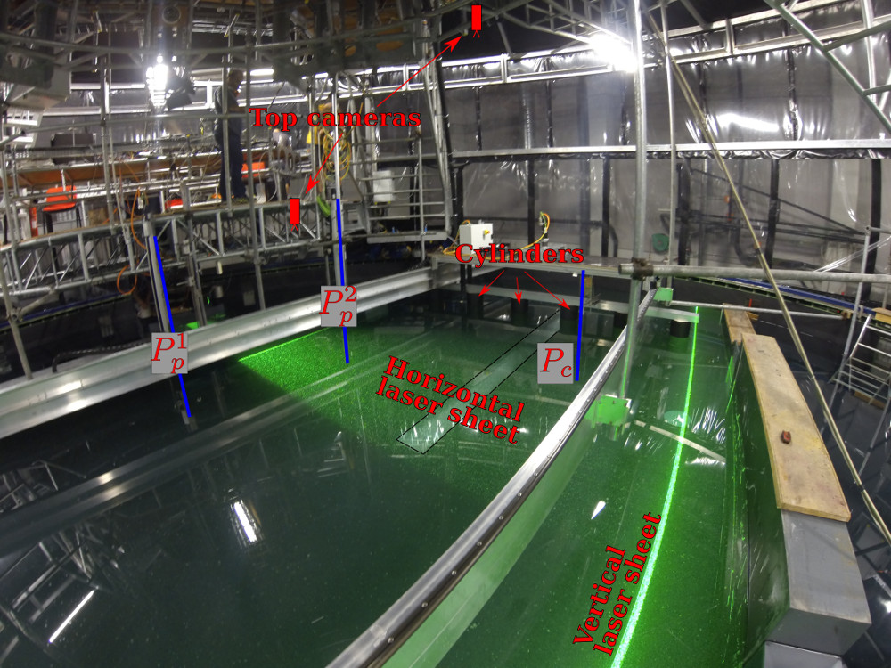
2 sets of experiments
Summer 2016 (a collaboration between KTH, Stockholm, Sweden and LEGI): we tried many things.
Summer 2017: focused on mixing without rotation
- larger horizontal cylinders (25 cm and 50 cm diameter)
- better measurements of the density profiles
- vertical cylinders (producing waves)
- alcool to decrease differences in refractive index (actually no alcool!)
Methods: introduction to open-science and open-source
- World Wide Web
- big data (storage, flux)
- companies (Youtube, Google)
- algorithms
- open-source (using in particular Python)
Open-source today
Big changes in how programs are developed:
- a lot of money (web, big companies as google or facebook and startups)
serious, good quality, good coding practices:
- distributed version control software (Git, Mercurial)
- forges for collaborative development (github, bitbucket, gitlab)
- issue tracker
- continuous integration
- documentation
- unittests
- benchmarking
new tools and environments (for example Python)
Open-science
Transparency in scientific methods and results
Openness to full scrutiny
Ease of reproducibility
No more "reinventing the wheel" - particularly in code development
More practical:
Doing sciences with open-source methods and tools
Share using the web
Remark: different stories and tools for different communities
Fluid mechanics not in advance... Dominance of Fortran and Matlab,
- good tools for few very specialized purposes
- but not plugged to the open-source and web dynamics
Python language and its scientific ecosystem for open-science
A well-thought language:
- dynamic
- generalist
- fast prototyping
- easy to learn and teach
- multi-platform
Scientific ecosystem: strong dynamics, rich and complicated landscape (many, many projects):
- rich Python standard library
- core scientific Python packages (ipython, jupyter, numpy, scipy, matplotlib),
- many specialized tools (oriented toward methods and goals),
- performance (cython, pythran, numba, ...)
- GPU, distributed computing
- visualisation (see this presentation, for fluid: Paraview, Visit, ...)
- symbolic math (sympy)
- scientific file format (h5py, h5netcdf, ...)
- statistics (statsmodels)
- automatization, Internet of Things, Microcontrollers
- image processing (scikit-image)
- database (SQL, NoSQL, ORM)
- Geographic Information System (Qgis)
- Artificial Intelligence, Machine Learning, Deep Learning
- GUI (PyQt, kivy, ...)
- web framework
- libraries by and for scientific communities (oriented towards subjects)
- fluid mechanics... only the very beginning of this trend...
Remark on a technological trend: exotic architecture for computers
Difficult to use efficiently (very specialized coding)
low-level languages versus high-level languages?


Tensorflow (deep learning library by Google)
$\rightarrow$ main APIs in Python
A contribution to open-science: the fluiddyn project
Open-source, documented, tested, continuous integration
- fluiddyn: base package containing utilities
- fluidlab: control of laboratory experiments
- fluidimage: scientific treatments of images (PIV)
- fluidfft: C++ / Python Fourier transform library (highly distributed, MPI, CPU/GPU, 2D and 3D)
- fluidsim: pseudo-spectral simulations in 2D and 3D
- fluidfoam: Python utilities for openfoam
- fluidcoriolis: running and analyzing experiments in the Coriolis platform
Main developpers:
- Pierre Augier (LEGI)
- Cyrille Bonamy (LEGI)
- Antoine Campagne (LEGI)
- Ashwin Vishnu (KTH)
- Julien Salort (ENS Lyon).
Studying mixing efficiency and stratified turbulence with experiments and open-science
The MILESTONE experiment: stratified and rotating turbulence in the Coriolis platform

- LEGI group: Pierre Augier, A. Campagne, J. Sommeria, S. Viboud, C. Bonamy, N. Mordant...
- KTH group (Stockholm, Sweden): E. Lindborg, A. Vishnu, A. Segalini
- Diane Micard (LMFA)
The MILESTONE experiment
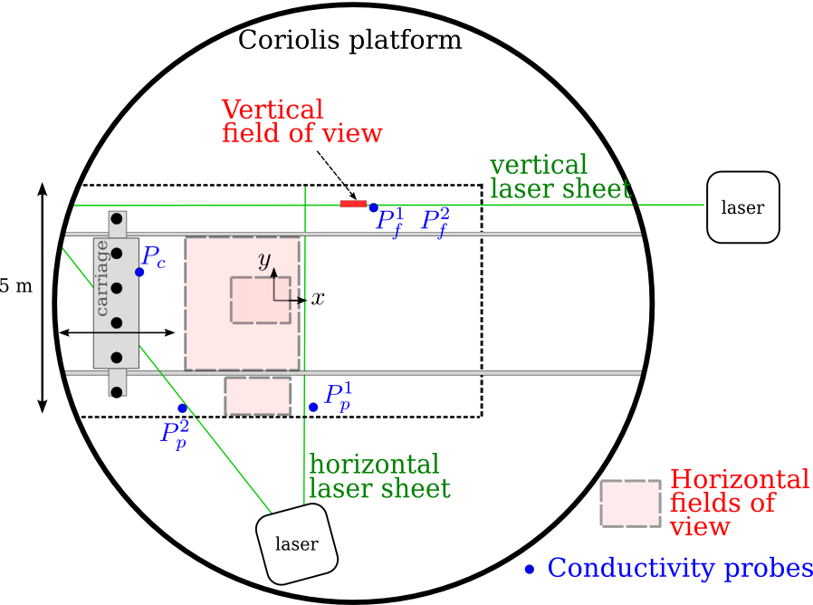 Top view (MILESTONE 2016)
A new carriage for the Coriolis plateform!
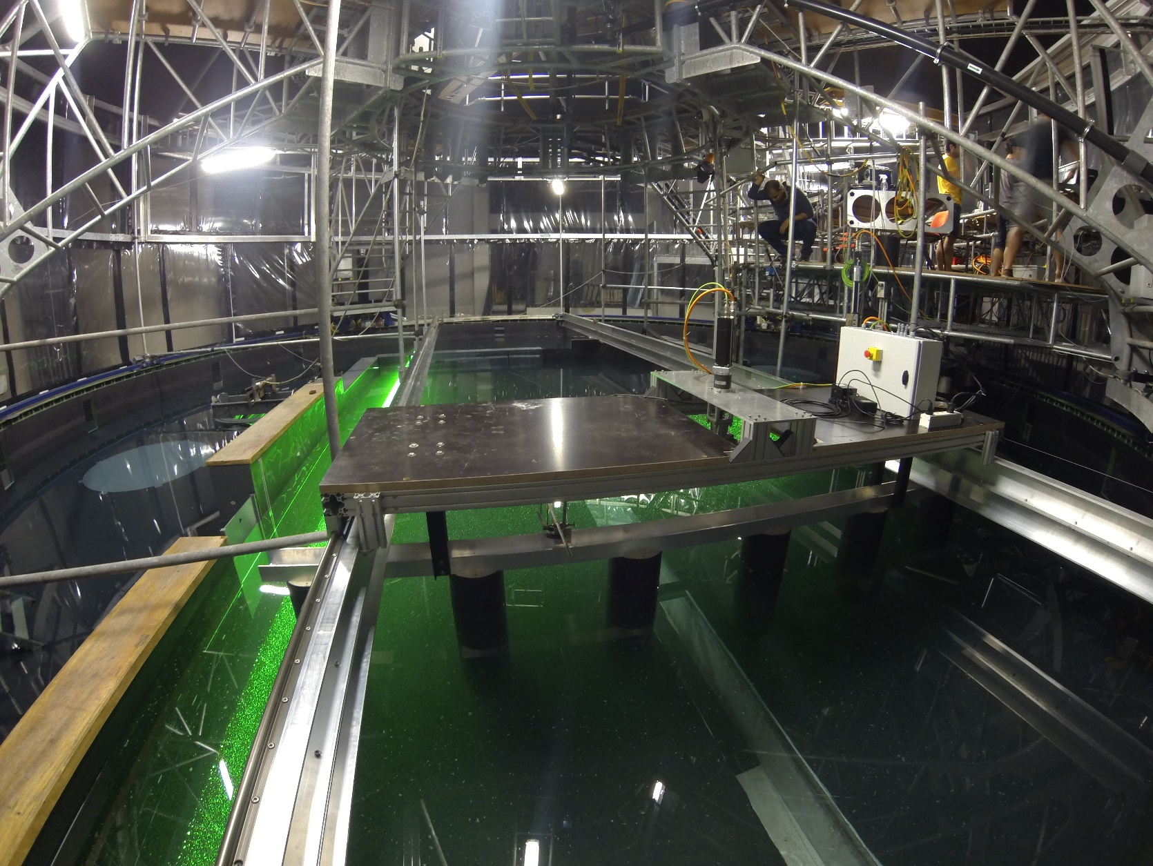
- 3 m $\times$ 1 m
- runs on tracks (13 m long)
- good control in position ($\Delta x<$ 5 mm) and in speed ($U< 25$ cm/s)
Measurements: PIV and probes (density, temperature)

(in collaboration with Julien Salors, ENS Lyon)
Physical experiments can be seen as the interaction of autonomous physical objects
For the MILESTONE experiments:
- moving carriage, motor (Modbus TCP), position sensor (quadrature signal)
probes attached to a transverses (Modbus TCP)
scanning Particle Image Velocimetry (PIV):
- oscillating mirror driven by an acquisition board
- cameras triggered by a signal produced by an acquisition board
Issue: control with computers the interaction and synchronization of the objects
(in collaboration with Julien Salors, ENS Lyon)
Physical experiments can be seen as the interaction of autonomous physical objects
- Object-oriented programming
- Very easy to write instrument drivers
- Automatic documentation for the instrument drivers
- Simple servers with the Python package
rcpy
Example for the carriage
motor.pyposition_sensor.pyposition_sensor_server.pyposition_sensor_client.pycarriage.pycarriage_server.pycarriage_client.py
A little bit of Graphical User Interface is easy, fun and useful. We use PyQt.
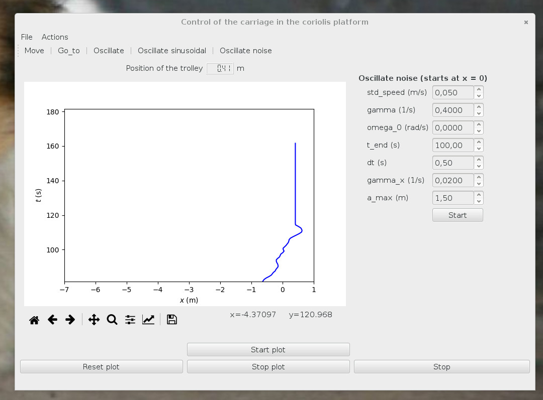
Remark: reusable code, here, random movement for another experiment.
How to estimate the mixing coefficient?
$$\Gamma = \frac{\eps_P}{\eps_K}$$Kinetic energy dissipation rate $\eps_K$:
$\eta$ very small: impossible to measure accuratly the velocity gradients
decay of kinetic energy after a stroke. Need many vector fields $\Rightarrow$ scanned horizontal PIV
APE dissipation rate $\eps_P$:
$\kappa$ smaller than $\nu$!
APE decay after one stroke...
long-term evolution of the stratification after many strokes $\Rightarrow$ density profiles
Processing of experimental data
Very large series of images and probe data $\Rightarrow$ calcul on the LEGI clusters
fluidimage: scientific treatments of images
(in collaboration with Cyrille Bonamy and Antoine Campagne, LEGI)
Many images (~ 20 To of raw data): embarrassingly parallel problem
- Clusters and PC, with CPU and/or GPU
- Asynchronous computations
- topologies of treatments
- IO and CPU bounded tasks are splitted
- compatible with big data frameworks as Storm
Efficient algorithms and tools for fast computation with Python (Pythran, Theano, Pycuda, ...)
Images preprocessing
2D and scanning stereo PIV
Utilities to display and analyze the PIV fields
- Plots of PIV fields (similar to PivMat, a Matlab library by F. Moisy)
- Calcul of spectra, anisotropic structure functions, characteristic turbulent length scales
Remark: we continue to use UVmat for calibration
Calcul of scanning PIV on the LEGI cluster
Example of scripts to launch a PIV computation:
from fluidimage.topologies.piv import TopologyPIV

params = TopologyPIV.create_default_params()

params.series.path = '../../image_samples/Karman/Images'
params.series.ind_start = 1
params.piv0.shape_crop_im0 = 32
params.multipass.number = 2
params.multipass.use_tps = True
# params.saving.how has to be equal to 'complete' for idempotent jobs
# (on clusters)
params.saving.how = 'complete'
params.saving.postfix = 'piv_complete'

topology = TopologyPIV(params, logging_level='info')
topology.compute()
Remark: parameters in an instance of fluiddyn.util.paramcontainer.ParamContainer. Much better than in text files or free Python variables!
- avoid typing errors
- the user can easily look at the available parameters and their default value
- documentation for the parameters (for example for the PIV topology)
Calcul of scanning PIV on the LEGI cluster
Remark: launching computations on cluster is highly simplified by using fluiddyn:
from fluiddyn.clusters.legi import Calcul7 as Cluster

cluster = Cluster()

cluster.submit_script(
    'piv_complete.py', name_run='fluidimage',
    nb_cores_per_node=8,
    walltime='3:00:00',
    omp_num_threads=1,
    idempotent=True, delay_signal_walltime=300)
Analysis and production of scientific figures
- For one experiments, a lot of different files for different types of data (txt and hdf5 files)
- Classes for experiments and types of data (for example probe data or PIV field).
from fluidcoriolis.milestone17 import Experiment as Experiment17
iexp = 21
exp = Experiment17(iexp)
exp.name
'Exp21_2017-07-11_D0.5_N0.55_U0.12'
print(f'N = {exp.N} rad/s and Uc = {exp.Uc} m/s')
N = 0.55 rad/s and Uc = 0.12 m/s
print(f'Rc = {exp.Rc:.0f} and Fh = {exp.Fhc:.2f}')
Rc = 11425 and Fh = 0.44
print(f'{exp.nb_periods} periods of {exp.period} s')
3 periods of 125.0 s
print(f'{exp.nb_levels} levels for the scanning PIV')
5 levels for the scanning PIV
Studying and plotting PIV data
from fluidcoriolis.milestone import Experiment
exp = Experiment(73)
cam = 'PCO_top'  # MILESTONE16
# cam = 'Cam_horiz'  # MILESTONE17
pack = exp.get_piv_pack(camera=cam)
piv_fields = pack.get_piv_array_toverT(i_toverT=80)
/home/pierre/16MILESTONE/Data_light/PCO_top/Exp73_2016-07-13_N0.8_L6.0_V0.16_piv3d/v_exp73_t080.h5
piv_fields = piv_fields.gaussian_filter(0.5).truncate(2)
piv = pack.get_piv2d(ind_time=10, level=1)
piv = piv.gaussian_filter(0.5).truncate(2)
piv.display()
_ = plt.xlim([-1.7, 0.5])
_ = plt.ylim([-1.3, 1.3])
piv.display()
_ = plt.xlim([-1., -0.])
_ = plt.ylim([-0.5, 0.5])
from fluidcoriolis.milestone.results_energy_budget import ResultEnergyBudgetExp
r = ResultEnergyBudgetExp(73, camera=cam)
iexp = 73; N = 0.8 rad/s; Uc = 16 cm/s
epsK = 5.49e-05 m^2 s^-3
urms = 3.14e-02 m/s
(urms/Uc)^2 = 4e-02 ; epsK/epsc = 3e-03
Fht = 1.0e-01 ; Rt = 1.3e+02
r.plot_energy_vs_time()
fig = plt.gcf()
fig.set_size_inches(12, 5, forward=1)
Fit of energy decay

$[F_h, \R]$ diagram from fit of kinetic energy decay

Density profiles
from fluidcoriolis.milestone17.time_signals import SignalsExperiment
signals = SignalsExperiment(iexp)
/fsnet/project/watu/2017/17MILESTONE/Data/Exp21_2017-07-11_D0.5_N0.55_U0.12
signals.plot_vs_times()
signals.plot_vs_times(corrected=1)
probe = signals.probes_profiles[0]
probe.plot_profiles(corrected=1)
signals.plot_profiles_probe_averaged(corrected=1, sort=1, extend=1, len_extend=0.005)
signals.plot_energy_pot_vs_time()
Mass conservation check:
max(m/m0 - 1) = 1.6755e-04
non-dimensional mixing: 0.001983362753471777
Dimensionless potential energy dissipation
$$ \frac{\eps_P}{(3\times10^{-3} U_c^3/D_c)}$$
Conclusions on mixing by stratified turbulence
- New experimental setup in the Coriolis platform with many new development and improvements
Experimental flow close to the strongly stratified regime!
We should be able to get strongly stratified turbulence by using alcool
Good measurements of the mixing (with MILESTONE17)
$\Rightarrow$ soon good evaluation of the mixing coefficient
- Many things to look at in the data (soon open)
Numerical simulations
Easier than experiments! :-)
fluidfft: unified API (C++ / Python) for Fast Fourier Transform libraries
- highly distributed, MPI,
- CPU and GPU,
- 2D and 3D
fluidsim: pseudo-spectral simulations in 2D and 3D
- highly modular (object oriented solvers)
- efficient (Cython, Pythran, mpi4py, h5py)
- inline data processing
Conclusions on open science
Science in fluid mechanics with open-source methods and Python
Open-data: data in auto-descriptive formats (hdf5, netcdf, ...) + code to use and understand the data
Development of open-source, clean, reusable codes (fluiddyn project)
Issues
- Collaborative dynamics? Adoption by the community? Developpers?
- Level in Python and coding in the community ! => Python training sessions in the lab and at university
