On Wednesday 31th of August, I gave a presentation at the IX International Symposium on Stratified Flows in Cambridge.

The title of my presentation is A comprehensive open dataset of stratified turbulence forced in vertical vorticity and the slides are here .

Moreover, Vincent Labarre and Nicolas mordant presented our work on Stratified turbulence forced in waves and Investigation of the spectral properties of stratified turbulence generated by waves in the Coriolis facility , respectively.

Abstract ¶

\(\newcommand{\R}{\mathcal{R}} \newcommand{\epsK}{{\varepsilon_{\!\scriptscriptstyle K}}} \newcommand{\epsA}{{\varepsilon_{\!\scriptscriptstyle A}}} \newcommand{\kmax}{k_{\max}}\) We present a new comprehensive open dataset of stratified turbulence forced in large horizontal vortices invariant over the vertical in a periodic domain with constant Brunt-Väisälä frequency \(N\) . More than 40 simulations were carried out with the ns3d.strat pseudo-spectral solver of the open-source CFD framework Fluidsim .

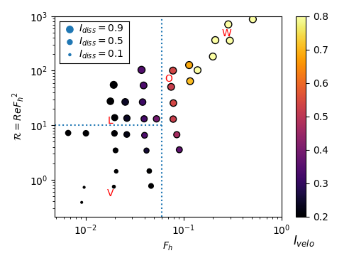
This dataset has 4 main particularities. (i) The horizontally invariant shear modes, which can represent more than half of the total energy in similar simulations, are cleanly removed from the dynamics. (ii) Large ranges of horizontal Froude \(F_h = \epsK /(N U_h^2) \in [0.007, 2]\) and buoyancy Reynolds \(\R = Re {F_h}^2 = \epsK / (\nu N^2)\) numbers are investigated, where \(U_h\) is the horizontal rms velocity, \(\epsK\) is the kinetic energy dissipation rate, and \(\nu\) is the viscosity. This dataset is thus adapted to investigate the different regimes of stratified flows forced with vortices, in particular the weakly stratified regime ( \(F_h > 0.1\) ) and the Layered Anisotropic Stratified Turbulence regime (LAST, \(F_h < 0.07\) and \(\R > 10\) ). (iii) Few simulations for the largest Reynolds numbers (necessary to reach large \(\R\) for very small \(F_h\) ) are badly resolved quasi-DNS ( \(\kmax \eta \simeq 0.5\) , with \(\eta\) the Kolmogorov lengthscale) with both standard viscosity and order 4 hyperviscosity.

fig_isotropy_coef_vs_FhR — Isotropy coefficients (left) and mixing coefficient (right), in a space set by R and F_h. Each point corresponds to one simulation. (left) Colors represent a large scale isotropy and markersize a small scale isotropy (see legend). The large and dark markers correspond to the LAST regime.

fig_mixing_coef_vs_Fh — Isotropy coefficients (left) and mixing coefficient (right), in a space set by R and F_h. Each point corresponds to one simulation. (left) Colors represent a large scale isotropy and markersize a small scale isotropy (see legend). The large and dark markers correspond to the LAST regime.

(iv) Statistical quantities like (1) spatial, temporal and spatio-temporal spectra and (2) spectral energy budget are provided. We will show how it will be easy for anyone to investigate stratified turbulence with this dataset by loading and plotting these quantities with our Python library Fluidsim.

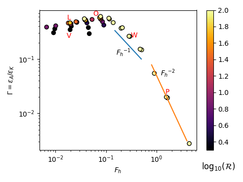
Different physical questions will be addressed in view of numerous geophysical applications. (i) Characterization of the different regimes (left figure), in particular through comparisons based on spatial and temporal spectra with theoretical results and in-situ measurements. (ii) Scaling laws for different averaged quantities like the mixing coefficient \(\Gamma=\epsA/\epsK\) (right figure), where \(\epsA\) is the potential energy dissipation rate. (iii) Presence and degree of nonlinearity of internal gravity waves through a spatio-temporal analysis.